Vector Search Performance Optimisation | Expert Tuning — Codersarts AI

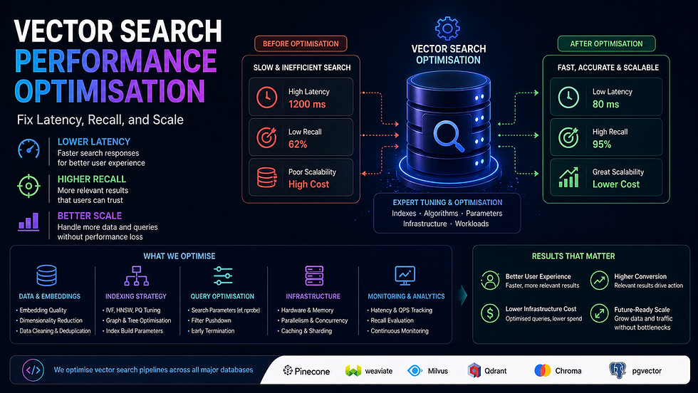
Vector Search Performance Optimisation — Fix Latency, Recall, and Scale

A vector search system that takes 2 seconds to respond is not a search system — it is a liability. Slow queries, poor recall, bloated memory, and indexes that fall over at scale are all fixable problems. But only if you know exactly which lever to pull.

At Codersarts, our engineers diagnose and fix vector search performance issues across every major platform — Pinecone, Weaviate, Qdrant, Milvus, FAISS, pgvector, and Redis. We tune indexes, fix recall quality, implement hybrid search, and migrate broken systems to the right architecture — with measured before/after benchmarks delivered with every engagement.

Whether your p99 query latency is 3 seconds or 300ms and needs to be 50ms, we have done it and we can do it for you.

< 50ms Target p99 query latency

10x Typical throughput gain

< 4h First response

24–72h Typical fix delivery

Measured Before/after benchmarks

Why Vector Search Gets Slow — The Most Common Root Causes

Most performance problems have a small set of root causes. We diagnose the exact one before touching anything — because the wrong fix makes it worse.

Symptom	Most Likely Root Cause	The Fix
Query latency > 500ms at < 1M vectors	Wrong index type (Flat instead of HNSW/IVF)	Rebuild index with HNSW — typical 20–100x speedup
Query latency degrades as index grows	HNSW ef_construction too low, M too small	Re-index with correct M and ef_construction params
High recall but very slow queries	ef (search-time param) set too high	Tune ef downward — same recall at 3–5x lower latency
Low recall — wrong results returned	Wrong distance metric for embedding model	Switch metric (cosine vs L2 vs dot) to match model
Filtered queries 10x slower than unfiltered	Post-filtering on large index (no pre-filter index)	Add payload/metadata index, switch to pre-filtering
Memory usage explodes at 10M+ vectors	HNSW in-memory for dataset too large	Quantization (PQ/SQ) or switch to IVF+HNSW hybrid
Slow ingestion blocking query performance	Upsert and query sharing same index lock	Separate ingestion and query paths, async upsert
Recall drops after adding new vectors	Index not rebuilt after large batch insert	Trigger index rebuild or use incremental HNSW update
Hybrid search slower than pure vector	BM25 and vector run sequentially, not in parallel	Parallelise retrieval paths, tune fusion weights
DB migration causing data loss or slowdown	Direct copy without re-indexing	Full re-embed + re-index with validation checks

What Our Performance Optimisation Covers

✓  HNSW M and ef_construction parameter tuning	✓  IVF nlist and nprobe optimisation
✓  Product Quantization (PQ) and Scalar Quantization (SQ)	✓  Distance metric correction (cosine / L2 / dot product)
✓  Metadata filtering index design (pre vs post filter)	✓  Hybrid search (vector + BM25) parallelisation
✓  Query-time ef / top-K tuning for latency vs recall	✓  Memory footprint reduction at scale
✓  Batch upsert vs real-time upsert architecture	✓  Sharding and replication for high-throughput reads
✓  Vector DB migration with zero data loss	✓  Before/after latency and recall benchmarks
✓  Load testing at 2x and 5x expected QPS	✓  Monitoring and alerting setup post-optimisation
✓  Connection pooling and client-side optimisation	✓  Query caching for frequent repeated queries

1.  HNSW Index Tuning

HNSW — the Most Powerful Index, the Most Misunderstood Parameters

HNSW (Hierarchical Navigable Small World) is the index algorithm behind the fastest vector search systems in production. It delivers sub-millisecond approximate nearest neighbour search at million-vector scale — but only if the three key parameters are set correctly for your data and query distribution.

The default parameters shipped by every vector DB are wrong for most production use cases. They are conservative defaults designed not to break — not to perform.

The Three HNSW Parameters That Control Everything

Parameter	What It Controls	Default (typical)	Correct Range	Impact of Wrong Value
M	Number of bi-directional links per node	16	8–64	Too low: poor recall. Too high: memory explodes, slow build
ef_construction	Candidates explored during index build	200	100–800	Too low: poor recall quality baked in at build time (not fixable at query time)
ef (search)	Candidates explored during query	50	50–500	Too low: poor recall. Too high: latency degrades 5–20x

What Our HNSW Tuning Covers

• Benchmark your current index: measure recall@1, @5, @10 and p50/p99 query latency as baselines

• M parameter sweep: test M = 8, 16, 32, 48 — find the point where recall plateaus vs memory cost

• ef_construction tuning: requires index rebuild — we script this to run overnight on your full dataset

• ef search-time tuning: no rebuild needed — tune until recall and latency targets are both met

• Platform-specific syntax: qdrant hnsw_config, weaviate vectorIndexConfig, pgvector SET hnsw.ef, milvus index_params

• Memory footprint calculation: project RAM requirement at 10x and 100x current vector count

• Index rebuild pipeline: automate rebuild on schema change or large batch insert with zero query downtime

• Delivered benchmark report: before/after recall@K and p50/p99 latency for every parameter combination tested

Full HNSW tuning service →

Our HNSW Index Tuning Help page covers parameter sweep methodology, platform-by-platform configuration syntax, rebuild automation, and memory projection calculations for Pinecone, Weaviate, Qdrant, Milvus, FAISS, and pgvector.

2.  IVF + PQ Quantization

IVF + PQ — When HNSW Memory Cost Becomes the Bottleneck

HNSW stores the full float32 vectors in memory. At 10 million 1,536-dimension vectors (OpenAI embedding size), that is approximately 59GB of RAM — beyond what most cloud instances provide affordably. Inverted File Index (IVF) combined with Product Quantization (PQ) compresses vectors to a fraction of that size with minimal recall loss.

IVF+PQ is the right architecture for datasets above 5–10 million vectors where memory cost is a constraint, or for on-device / edge deployment where RAM is strictly limited.

What Our IVF + PQ Implementation Covers

• IVF nlist tuning: number of Voronoi cells — rule of thumb sqrt(n_vectors), but must be tested empirically

• nprobe tuning: cells searched at query time — controls the recall vs latency tradeoff after IVF

• PQ m (subvectors) and nbits configuration: more subvectors = better recall, more memory

• Scalar Quantization (SQ8, SQ4) as a simpler alternative to PQ with less recall loss

• IVFPQ vs IVFFlat vs HNSW+PQ comparison benchmark on your actual data

• Memory footprint comparison: HNSW vs IVF+PQ at your target vector count

• FAISS IndexIVFPQ setup and GPU acceleration for billion-scale datasets

• Milvus IVF_PQ index configuration and training pipeline

• Qdrant scalar quantization and product quantization configuration

• Quantization-aware retrieval: compensate for recall loss with higher nprobe

Full IVF + PQ service →

Our IVF + PQ Quantization Help page covers memory vs recall tradeoff benchmarks at 1M, 10M, 100M, and 1B vector scales, platform-specific configuration, and a quantization strategy decision framework.

3.  Hybrid Search (Vector + BM25) Implementation

Hybrid Search — Better Recall Than Either Keyword or Vector Alone

Pure vector search misses exact matches — product SKUs, person names, code identifiers, and domain-specific terms that embeddings generalise away. Pure BM25 keyword search misses semantic meaning — it cannot match 'automobile' to 'car'. Hybrid search combines both, consistently outperforming either approach alone on real-world retrieval benchmarks.

The tricky part is not running both — it is the fusion layer that merges two differently-scaled score lists into a single ranked result. Done wrong, one signal completely drowns the other.

What Our Hybrid Search Implementation Covers

• Sparse retrieval: BM25 via Elasticsearch, OpenSearch, or native sparse vectors (Qdrant, Weaviate)

• Dense retrieval: your existing vector search pipeline

• Reciprocal Rank Fusion (RRF): the most robust score fusion method — no score normalisation needed

• Linear combination fusion: weighted sum of normalised vector and BM25 scores, weight tuned on your eval set

• Weaviate hybrid search: alpha parameter tuning (0=BM25 only, 1=vector only, 0.7=optimal for most)

• Qdrant sparse + dense vector setup: SPLADE or BM25 sparse vectors alongside dense

• Pinecone hybrid search: sparse-dense index with BM25 sparse encoder integration

• Elasticsearch kNN + BM25 hybrid: script_score with kNN and BM25 combined query

• Parallel retrieval: run BM25 and vector retrieval concurrently to avoid latency doubling

• Reranker as third stage: cross-encoder reranks the fused candidates for maximum precision

• A/B evaluation: measure NDCG@10 for pure vector, pure BM25, and hybrid — show the improvement

Full hybrid search service →

Our Hybrid Search Implementation page covers RRF vs linear fusion decision framework, platform-specific sparse vector setup, parallel retrieval architecture, and measured NDCG benchmarks comparing all three approaches on standard datasets.

4.  Metadata Filtering Optimisation

Metadata Filtering — The Hidden Performance Killer in Production Vector Search

Metadata filtering lets you restrict vector search to a subset of your index — 'return the most similar products in the Electronics category priced under ₹5,000'. In theory, this should be faster than searching the full index. In practice, a naive post-filter implementation makes queries 10–50x slower when the filter is highly selective.

The root cause: if you retrieve the top-1000 vectors and then apply the filter, most queries with selective filters discard 990 results and return almost nothing. The fix is pre-filtering — filtering the index before the ANN search, not after. But pre-filtering requires a payload index on the filter fields, and most teams skip this step.

What Our Metadata Filtering Optimisation Covers

• Payload index creation: keyword, integer range, geo, and nested field indexes on filter columns

• Pre-filter vs post-filter architecture: diagnose which your current system uses and fix if needed

• Filter selectivity analysis: estimate what fraction of the index each filter returns — drives strategy

• Qdrant payload indexes: create_payload_index for keyword, integer, float, and geo fields

• Weaviate where filter with pre-filtering on indexed properties

• Pinecone metadata filter: design namespace vs metadata tradeoff for your filter patterns

• pgvector hybrid SQL+vector queries: combine WHERE clause pre-filtering with <=> similarity operator

• Milvus partition key design for high-cardinality filter fields

• Filter-aware HNSW: ef parameter adjustment when filter selectivity is < 10%

• Query latency benchmark: filtered vs unfiltered at p50/p99 before and after optimisation

Full metadata filtering service →

Our Metadata Filtering Optimisation page covers filter selectivity mathematics, pre-filter vs post-filter decision trees, payload index design patterns for each platform, and before/after latency benchmarks on high-selectivity filter queries.

5.  Vector DB Latency Debugging

Latency Debugging — Finding the Exact Millisecond Being Wasted

When your vector search is slow in production, there are eight possible bottlenecks — and they require completely different fixes. Without profiling each layer, you are guessing. We instrument your full query path, measure each component independently, and find the exact bottleneck before recommending any fix.

The Eight Latency Layers We Profile

Layer	What We Measure	Typical Contribution	Common Fix
Client → DB network	TCP round-trip time	5–50ms	Move client closer to DB region
Connection pool	Time waiting for available connection	10–200ms	Increase pool size, add pgbouncer
Query embedding time	Time to embed the query text	20–100ms	Cache frequent query embeddings
ANN search (index scan)	Time for HNSW/IVF graph traversal	1–500ms	Tune ef, rebuild index with higher M
Metadata filter	Post-filter or pre-filter execution	1–5,000ms	Add payload index, switch to pre-filter
Result fetch + deserialise	Time to retrieve and parse result data	5–50ms	Reduce returned fields, use projection
Reranker (if present)	Cross-encoder re-scoring	50–500ms	Reduce candidates, use faster model
Application processing	Code between DB response and API return	10–100ms	Profile app code, async where possible

What Our Latency Debugging Covers

• End-to-end request tracing: instrument each layer with timestamps and log to a structured format

• p50, p95, p99 latency breakdown by layer — find the long tail, not just the average

• Load test at 1x, 2x, and 5x expected QPS — identify where latency degrades non-linearly

• Connection pool profiling: measure pool saturation, queue depth, and connection acquisition time

• Query embedding cache analysis: what % of queries could be served from cache

• Index scan profiling: platform-specific explain/profile commands to inspect ANN traversal

• Reranker latency profiling: measure candidates-in vs latency to find optimal top-K before rerank

• Fix implementation: we do not just identify the bottleneck — we fix it and measure the improvement

• Delivered report: per-layer latency before and after, with annotated trace for each bottleneck fixed

Full latency debugging service →

Our Vector DB Latency Debugging page covers our 8-layer profiling methodology, platform-specific profiling commands, load testing setup, and a latency budget worksheet that lets you set targets per layer before you start optimising.

6.  Vector DB Migration Help

Vector DB Migration — Move Platforms Without Losing Data, Recall Quality, or Uptime

Teams migrate vector databases for three reasons: they outgrew a free tier, they chose the wrong platform early and are paying for it, or their requirements changed (on-prem security, multi-tenancy, cost). A migration done wrong means re-embedding millions of documents, corrupted indexes, and downtime that kills production.

We have migrated teams from ChromaDB to Pinecone, FAISS to Qdrant, Pinecone to Weaviate, pgvector to Milvus, and every other combination. The key is a structured migration plan with validation at every step — not a bulk copy that you hope works.

Common Migration Paths We Handle

From	To	Why Teams Migrate	Our Typical Delivery
ChromaDB	Pinecone / Qdrant	Outgrew local setup, need cloud scale	3–5 days
FAISS	Qdrant / Weaviate	Need filtering, multi-tenancy, managed hosting	3–7 days
Pinecone	Qdrant / Weaviate	Cost reduction, self-hosting, more control	5–7 days
pgvector	Pinecone / Milvus	Scaling beyond PostgreSQL vector capabilities	5–10 days
Weaviate v3	Weaviate v4	Breaking API changes in major version upgrade	2–4 days
Any DB	pgvector	Consolidate to existing PostgreSQL infrastructure	3–5 days
FAISS	Milvus / Zilliz	Billion-scale, GPU acceleration, managed ops	7–14 days

What Our Migration Service Covers

• Migration feasibility assessment: can vectors transfer directly or do we need to re-embed?

• Schema mapping: map source collection/index structure to target platform's data model

• Vector export pipeline: batch export from source with ID, vector, and metadata preservation

• Target setup: create index, configure schema, tune HNSW/IVF parameters on target before import

• Batch import with validation: import in chunks, verify vector count and spot-check recall after each batch

• Dual-write period: write to both old and new DB during cutover to catch any discrepancies

• Recall quality validation: run 100 benchmark queries on both source and target, compare top-5 results

• Zero-downtime cutover: switch application traffic to new DB with instant rollback capability

• Post-migration monitoring: watch error rates and latency for 48h after cutover

• Full migration runbook document delivered — so you can repeat the process yourself

Full migration service →

Our Vector DB Migration Help page covers every platform combination, dual-write cutover patterns, recall validation methodology, and a migration risk assessment checklist you can use before committing to a platform change.

Performance Targets — What Good Looks Like

Before we start any optimisation engagement, we agree on target metrics. Here are the benchmarks we aim for across common vector DB setups:

Setup	Dataset Size	Target p99 Latency	Target Recall@10	Notes
HNSW (Qdrant Cloud)	1M vectors	< 20ms	> 95%	Achievable without quantization
HNSW (Weaviate Cloud)	5M vectors	< 50ms	> 93%	With metadata pre-filtering
HNSW (Pinecone Serverless)	10M vectors	< 100ms	> 92%	With namespace isolation
IVF+PQ (FAISS GPU)	100M vectors	< 10ms	> 88%	With nprobe=64
pgvector HNSW	1M vectors	< 30ms	> 93%	With proper index params + connection pool
Milvus IVF_HNSW	50M vectors	< 50ms	> 91%	With partition pruning
Hybrid (Qdrant sparse+dense)	5M vectors	< 80ms	> 96%	Hybrid typically beats pure vector recall

Not hitting these numbers?

Share your current latency and recall measurements and we will identify the gap and the fix. Free 15-minute diagnosis call — no commitment required.

Our Performance Optimisation Process

Phase	What We Do	Output
1.  Baseline measurement	Measure current p50/p99 latency, recall@5/10, QPS, memory usage — no guessing	Baseline benchmark report
2.  Root cause diagnosis	Profile each layer of the query path, identify the primary bottleneck	Bottleneck diagnosis doc
3.  Fix proposal	Recommend the minimum set of changes to hit your targets — no over-engineering	Optimisation proposal
4.  Implementation	Apply fixes: parameter tuning, index rebuild, query rewrite, schema change	Optimised system
5.  Post-fix benchmark	Re-run the full benchmark suite — same queries, same data, measure improvement	Before/after benchmark report
6.  Load test	Simulate 2x and 5x expected QPS — confirm performance holds under load	Load test report
7.  Monitoring setup	Add latency and recall alerting so you catch degradation before users do	Monitoring dashboard

Why Teams Choose Codersarts for Vector Search Optimisation

✓  We benchmark before we touch anything	✓  We fix root causes — not symptoms
✓  All six major vector DBs covered	✓  HNSW, IVF, PQ, hybrid — all index types
✓  Delivered with before/after benchmark report	✓  Load tested at 2x and 5x expected QPS
✓  NDA available before sharing your architecture	✓  Monitoring setup included post-optimisation
✓  Migration help if platform change is needed	✓  First response in 4 hours, fix in 24–72 hours
✓  India-based pricing, production-grade quality	✓  Post-delivery support retainer available

Frequently Asked Questions

Q:  My vector search query takes 800ms. Where do I start?

A:  Start by profiling — not guessing. We instrument your query path and measure each layer independently: embedding time, connection pool wait, ANN scan, filter execution, result fetch, and application processing. In our experience, 80% of cases have a single dominant bottleneck. Once we find it, the fix is usually a parameter change or index rebuild — not an architecture rewrite.

Q:  I tuned HNSW ef and it made recall worse. What went wrong?

A:  Lowering ef at search time always reduces recall — that is the tradeoff. If your ef_construction was set too low at index build time, no amount of ef tuning at query time recovers that recall. The fix is a full index rebuild with higher ef_construction. We script this to run on your dataset and benchmark the result.

Q:  Our filtered queries are much slower than unfiltered. Is this normal?

A:  It is common but not normal — it is fixable. The cause is almost always post-filtering: your system retrieves the top-N vectors and then filters, which means highly selective filters return almost nothing and require retrieving far more candidates to compensate. The fix is adding a payload index on your filter fields and switching to pre-filtering. We have seen 20–50x speedups from this change alone.

Q:  We are at 15 million vectors and memory is our constraint. What are our options?

A:  Three options in order of impact: (1) Scalar Quantization — reduces memory by 4x with < 5% recall loss, no code change. (2) Product Quantization — reduces memory by 8–16x with 5–15% recall loss, requires re-indexing. (3) IVF+PQ — reduces memory by 16–32x for datasets where recall trade-off is acceptable. We benchmark all three on your data and recommend based on your recall requirements.

Q:  We want to migrate from Pinecone to Qdrant to reduce costs. How long does it take and is it risky?

A:  For a typical Pinecone index, migration takes 5–7 days and is low risk if done correctly. The risk comes from skipping validation steps — transferring vectors without verifying recall quality on the target. We use a dual-write period and run benchmark queries on both systems before cutting over traffic, so you have a tested rollback option at every stage.

Q:  How do I know if hybrid search will actually improve results for my use case?

A:  We run a controlled benchmark before implementing: take 50–100 representative queries from your real traffic, run them through pure vector search, pure BM25, and hybrid (with RRF fusion), then measure NDCG@10 for each. In our experience, hybrid outperforms pure vector on most real-world datasets — but we measure it on your data, not on a synthetic benchmark.

Q:  Can you optimise a pgvector setup running on Supabase?

A:  Yes. pgvector on Supabase has several specific constraints — connection pool limits via pgbouncer, the cost of HNSW index builds on shared infrastructure, and query planning decisions the Postgres planner makes around the <=> operator. We have tuned Supabase pgvector setups extensively and know exactly which parameters to adjust and which Supabase tier to target.

Vector search too slow, recall too low, or costs out of control? Let us fix it.

📋  Submit Performance Brief Share your latency issue. First response in 4 hours.

📞  Free Performance Audit Call 15 min. We diagnose your bottleneck live.

💬  WhatsApp Us Urgent latency issue in production? Message now.

Get a Free Scope Quote — 4-Hour Response

---

Other Vector Database Services We Offer

Performance optimisation touches every layer of the vector search stack. If you need help with a related area — building a pipeline from scratch, migrating platforms, or preparing for an interview — the pages below cover each in full.

Performance Optimisation Sub-services

→  HNSW Index Tuning Help — M, ef_construction, ef sweep, platform-specific syntax, recall benchmarks

→  IVF + PQ Quantization Help — memory vs recall tradeoffs, nlist/nprobe tuning, FAISS and Milvus config

→  Hybrid Search (Vector + BM25) Implementation — RRF fusion, sparse+dense setup, NDCG benchmarks

→  Metadata Filtering Optimisation — payload indexes, pre vs post filter, selectivity analysis

→  Vector DB Latency Debugging — 8-layer profiling, load testing, before/after benchmark report

→  Vector DB Migration Help — every platform combination, dual-write cutover, zero-downtime migration

Build & Implement

→  Vector Database Implementation Help — full setup: Pinecone, Weaviate, Qdrant, Milvus, pgvector, ChromaDB, Redis

→  RAG Pipeline Development — LangChain, LlamaIndex, any LLM, production-ready RAG builds

→  Embedding Pipeline Development — batch, async, cached, multi-modal embedding pipelines

→  Reranking Implementation Help — Cohere, cross-encoders, bge-reranker for better retrieval quality

Career & Architecture

→  Vector DB Job Support & Interview Preparation — system design rounds, HNSW questions, ML engineer interviews

→  Vector Database Architecture Design for Startups — DB selection, scaling plan, cost modelling

→  Vector DB Cost Optimisation & Scaling Plan — reduce spend at scale without sacrificing recall

Not sure which service fits your problem? Describe your symptoms on our contact page and we will diagnose the right fix.

Codersarts — Vector Search Performance Experts  |  ai.codersarts.com

---

Keywords: HNSW index tuning, vector search latency, IVF PQ quantization, hybrid search implementation, metadata filtering optimisation, vector DB migration, vector search slow fix