

How to Build a Predictive Maintenance and Remaining Useful Life Pipeline for Industrial Equipment

Predictive maintenance is often presented as a chart that turns red just before a machine fails. The real engineering problem is more demanding: histories from the same asset must not leak across data splits, sensor quality and operating conditions must be validated, uncertainty must be visible, and a forecast must pass through an approved maintenance policy before it becomes a work order.
This tutorial builds a compact but complete remaining useful life (RUL) pipeline. We will simulate a run-to-failure fleet, produce rolling sensor features, train a regularized regression model, calibrate a prediction interval on separate assets, evaluate planning and urgent-review windows, expose a FastAPI service, and package the system in Docker.
Every sensor record is synthetic. The results verify the tutorial implementation only; they are not maintenance advice or evidence that the model is safe for industrial use.
Technology stack: Python, NumPy, FastAPI, Pydantic, Pytest, Docker, and GitHub Actions.
What we are building
Our reference path keeps five concerns separate:
Asset sensing: load, RPM, vibration, temperature, and pressure.
Data quality: asset identity, timestamps, units, freshness, range, and missing values.
RUL model: a point estimate from a 12-cycle feature window.
Uncertainty and policy: a calibrated interval and decision state.
Maintenance execution: planner review and work-order systems.

The API returns a response shaped like this:
{
  "asset_id": "asset-050",
  "observed_cycle": 137,
  "model_version": "ridge-rul-conformal-v1",
  "predicted_rul_cycles": 0.0,
  "lower_bound_cycles": 0.0,
  "upper_bound_cycles": 10.896,
  "decision": "urgent_review",
  "top_drivers": [
    {"feature": "vibration_mean", "contribution_cycles": -17.961}
  ]
}
The exact feature contributions are sample-specific. They explain the arithmetic of this linear model, not the physical cause of degradation.
Why this is a timely industrial AI topic
The World Economic Forum identifies advanced manufacturing as one of the industries expecting especially broad AI adoption. NIST's 2026 smart-manufacturing roadmap emphasizes measurement science, validation, trustworthy AI, and deployment practices. NIST also operates a program on monitoring, diagnostics, and prognostics for manufacturing operations. Together, these sources point to demand for systems that connect ML with reliability engineering and operations—not only model prototypes. See the WEF industry analysis, NIST smart-manufacturing roadmap, and NIST monitoring, diagnostics, and prognostics program.
After completing this local tutorial, NASA's C-MAPSS turbofan simulation is a useful public run-to-failure dataset for a more advanced experiment. The official catalog describes multiple multivariate time series, operating conditions, sensor noise, and progressive faults: NASA C-MAPSS dataset catalog.
Prerequisites
Python 3.11 or newer
Docker Desktop or another Docker engine for container validation
Git
Familiarity with basic Python and HTTP APIs
Enter the companion project and create an environment:
cd examples/industrial-predictive-maintenance-rul
python -m venv .venv
Activate it on Windows PowerShell:
.venv\Scripts\Activate.ps1
On macOS or Linux:
source .venv/bin/activate
Install dependencies:
python -m pip install --requirement requirements-dev.txt
Step 1: Define the prediction and action contract
RUL is meaningful only when its unit and operational decision are precise. Before modeling, document:
the component and failure mode;
whether RUL means cycles, operating hours, starts, distance, or calendar time;
the observation point and minimum useful warning horizon;
the maintenance action, lead time, spare-part constraint, and responsible planner;
the cost of a missed warning and of unnecessary early maintenance;
what happens when data are stale, incomplete, out of range, or outside the trained regime.
The sample caps RUL at 100 cycles and uses three policy states:
healthy when the conservative lower bound is above 30 cycles;
plan_maintenance when the lower bound enters the 30-cycle planning window;
urgent_review when the point estimate is at most 10 cycles or the lower bound is at most 5.
These are tutorial thresholds, not maintenance recommendations.
Step 2: Generate an asset-separated fleet
Run:
python scripts/generate_dataset.py
The script creates 7,980 rows for 60 assets. Each asset has a randomized failure cycle and operating phase. As the synthetic asset approaches failure, vibration and temperature rise while pressure falls. Load, RPM, noise, and asset baselines add variation.
The split is performed by complete asset:
Split | Assets | Purpose |
Train | 40 | Fit feature scaling and model weights |
Calibration | 10 | Calibrate the residual interval |
Test | 10 | Final untouched evaluation |
This avoids a common leakage bug: putting early cycles of the same machine in training and later cycles in testing. The model could then memorize asset-specific baselines and appear much stronger than it is on a new machine.
The generated schema is intentionally simple:
asset_id,split,cycle,failure_cycle,load,rpm,vibration,temperature,pressure,target_rul
asset-000,train,1,147,0.71,1842.2,0.39,52.1,5.29,100
failure_cycle exists because this is simulated run-to-failure data. It is used to generate labels, never as a model input.
Step 3: Build time-aware feature windows
src/maintenance_ai/data.py groups records by asset, sorts them by cycle, and turns each 12-cycle window into:
current cycle;
current and mean load;
current and mean RPM;
current, mean, and slope of vibration;
current, mean, and slope of temperature;
current pressure and pressure slope.
The slope is calculated only from observations available up to the prediction cycle. This matters in historical backtesting: a feature pipeline must reproduce the information that would really have been available at that timestamp.
Real projects also need an explicit feature contract for units, sampling rate, aggregation, imputation, late events, time zones, sensor replacements, and post-maintenance resets. Training and serving must execute the same contract.
Step 4: Train an explainable baseline
Run:
python scripts/train.py
The code standardizes the 13 features and fits ridge regression. Ridge is a useful first baseline because it is fast, inspectable, and resistant to unstable coefficients when rolling features are correlated. A complex recurrent network or transformer should earn its operational cost by outperforming strong time-aware baselines on representative data.
The deterministic run created 1,628 training windows and 417 calibration windows. The model artifact records feature means, standard deviations, coefficients, intercept, interval radius, RUL cap, feature schema, and model version.
Step 5: Calibrate uncertainty on separate assets
A point estimate of 18 cycles does not say whether plausible error is 2 cycles or 25. The sample computes absolute errors on the 10 calibration assets and takes the 90th-percentile residual as the interval radius.
The current run produced:
target coverage        90%
interval radius        10.8958 cycles
For a prediction of 42 cycles, the displayed interval would be approximately 31.1 to 52.9 cycles after applying the 0–100 bounds.
This residual interval is a compact tutorial technique. Production uncertainty may vary by horizon, asset type, operating regime, failure mode, and data quality. Evaluate conditional coverage across those segments; good average coverage can still hide unreliable subgroups.
Step 6: Evaluate prediction and decision behavior
Run:
python scripts/evaluate.py
The script scores 418 windows from 10 held-out assets. The verified result is:
Metric | Result |
MAE | 4.963 cycles |
RMSE | 6.2763 cycles |
90% prediction-interval coverage | 91.63% |
Recall inside actual ≤30-cycle maintenance window | 99.06% |
Recall inside actual ≤10-cycle urgent window | 100.0% |
False urgent rate when actual RUL >30 | 0.0% |

The easy synthetic degradation pattern makes these results cleaner than real equipment data. The value of the exercise is the evaluation shape: prediction error, uncertainty coverage, actionable-window recall, and false-alert behavior are all checked on unseen assets.
The saved prediction trace shows how the forecast evolves for one held-out asset:
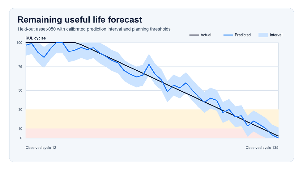
A production report should add lead-time distribution, precision of alerts, calibration plots, workload impact, downtime avoided, maintenance cost, and per-segment confidence intervals. It should also compare with calendar-based service, alarm thresholds, and reliability-engineering baselines.
Step 7: Run tests, including failure paths
Execute:
python -m pytest
The nine tests verify:
train, calibration, and test asset IDs are disjoint;
predictions and intervals remain inside their valid bounds;
a late-life window forecasts less RUL than an early window for the same asset;
the late-life demo routes to urgent review;
feature contributions reconstruct the raw linear score;
evaluation metrics satisfy tutorial guardrails;
health, readiness, known-asset, and unknown-asset API behavior.
The unknown-asset case returns HTTP 404. In production, equally explicit behavior is needed for stale windows, missing required sensors, unit mismatch, impossible values, duplicated events, and an unavailable model artifact.
Step 8: Serve the model with FastAPI
Start the service on PowerShell:
$env:PYTHONPATH="src"
uvicorn maintenance_ai.api:app --host 0.0.0.0 --port 8080
Verify readiness:
curl http://localhost:8080/readyz
Expected structure:
{
  "status": "ready",
  "model": "ridge-rul-conformal-v1",
  "demo_assets": 3
}
Request a forecast:
curl -X POST http://localhost:8080/v1/forecast \
  -H "Content-Type: application/json" \
  -d '{"asset_id":"asset-050"}'
The allow-listed demo assets are asset-050, asset-054, and asset-059. A real service should read an authenticated, point-in-time feature window from governed storage rather than loading a CSV into memory.
Step 9: Package the service safely
Generate the model artifact first, then build and run:
docker build -t maintenance-rul:1.0.0 .
docker run --rm -p 8080:8080 maintenance-rul:1.0.0
The Dockerfile uses a multi-stage build, an unprivileged runtime user, health checking, and a narrow copy set. For a real release, also pin the base image digest, scan the image and dependencies, generate an SBOM, sign the image, keep model provenance, and promote the same immutable image digest through staging and production.
Step 10: Add CI and release evidence
The included GitHub Actions workflow runs:
checkout → install → generate fleet → train → evaluate → test → docker build
That makes a public tutorial reproducible. For a production system, CI should validate code and packaging against a versioned test fixture. Model training normally belongs in a governed ML pipeline with immutable data references, lineage, approval criteria, and registered artifacts. A release record should bind together code commit, feature version, data snapshot, model, interval calibration, policy configuration, container digest, tests, and approver.
Step 11: Connect forecasts to maintenance operations responsibly
Validate telemetry first
Check asset identity, timestamp order, sample frequency, units, sensor calibration, missingness, range, flatline behavior, spikes, and operating regime. A model should not produce a normal-looking number from invalid telemetry.
Preserve event history
Capture inspections, maintenance actions, replaced components, downtime, load conditions, and confirmed failure modes. Without these outcomes, the team cannot tell whether an alert was useful or merely correlated with a maintenance event.
Keep prediction and policy separate
The model estimates RUL and uncertainty. A versioned policy decides whether to monitor, plan, or escalate. This separation lets reliability teams change lead-time rules without silently changing model behavior.
Include planners and reliability engineers
Show the recent sensor history, point estimate, interval, data-quality status, model version, and comparable cases. Record the planner's disposition. Feature contributions can support debugging, but they must not be presented as causal diagnosis.
Monitor outcomes
Track data-quality failures, input drift, residuals when outcomes become available, interval coverage, actionable lead time, alert precision and recall, planner acceptance, missed failures, premature maintenance, downtime, and financial value.
Common mistakes
Randomly splitting rows
Windows from the same asset share baseline behavior and adjacent measurements. Split by asset and time according to the intended deployment.
Training only on failed assets
Operational fleets contain right-censored assets that have not failed. Ignoring them can bias the population and the learned lifetime distribution. Use survival-analysis or censored-learning methods where appropriate.
Equating feature importance with root cause
A high vibration contribution says how the model calculated its score. It does not prove that vibration caused the failure.
Using one interval for every condition
Average calibration can hide poor uncertainty under rare loads, sites, equipment types, or failure modes. Report conditional coverage.
Automating work orders immediately
First run in shadow mode, review alerts with planners, measure lead time and false positives, and validate safety and cybersecurity boundaries.
Production extensions
Replace the generator with approved NASA C-MAPSS data or governed historian exports.
Add data-contract validation and operating-regime features.
Compare ridge regression with gradient boosting, temporal convolution, and survival models.
Add asymmetric or quantile intervals and evaluate conditional coverage.
Introduce a point-in-time feature store and model registry.
Add shadow deployment, policy simulation, drift monitoring, and rollback.
Integrate an approved maintenance planner workflow and measure real outcomes.
How Codersarts can help
Codersarts can help industrial teams identify high-value predictive-maintenance use cases, audit historian and work-order data, build time-series ML baselines, establish asset-safe validation, design MLOps and monitoring, and provide dedicated AI engineering expertise. A responsible engagement starts with data and decision feasibility before promising automated maintenance.
Contact: contact@codersarts.com
Product | Link | Description |
Codersarts | Coding and mentorship platform | |
Build | Build SaaS, MVPs, and products | |
Labs | Product development and solutions | |
AI | AI solutions and development | |
Dev | Developer tutorials and resources |
Explore the Codersarts Identity Verification API.


Comments